Disruptions pose a significant threat to the operation of future high-performance tokamaks. During a shot, the plasma control system must be able to predict a disruption with sufficient warning time to execute a response. However, deciding which response is best depends on how much warning time is given. For example, triggering disruption mitigation systems such as massive gas injection (MGI) can be done rapidly, but comes at a cost. While MGI radiates a significant fraction of the energy in the plasma, there is still damage caused by heat conduction to the divertor and electromagnetic forces on structural materials. A less aggressive action would be safely ramping down the plasma. This causes no incident damage but takes considerably longer.
Providing the plasma control system with the expected time to disruption would allow it to take actions which have the least amount of risk. This time-to-event prediction is a common application of machine learning, and there are many tools which have been developed in other fields for this purpose. The goal of this project is to benchmark these tools against presently implemented disruption predictors and determine differences in performance using metrics relevant to tokamak operation.
Many presently-implemented disruption predictors use a binary classifier, such as a random forest [Rea2019]. The time series data is represented as a collection of \(N\) tuples \(\{\vec x_i, d_i\}^N_{i=1}\), composed of feature vectors and labeled as ‘disruptive’ or ‘non-disruptive’. This labeling is determined by a class time \(\Delta \tau_\mathrm{class}\) before a disruption. After the model is trained, a new feature vector \(\vec x\) can be given to the model as input, and the output is the probability that the feature vector should be labeled as disruptive. Assuming that the probability of a disruption is uniformly distributed in the class time, the probability of a disruption occurring over some arbitrary time interval \(\Delta t\) is \(P_D(\vec x)\frac{\Delta t}{\Delta \tau_\mathrm{class}}\), and similarly the probability that no disruption occurs over that same time interval is \((1-P_D(\vec x)\frac{\Delta t}{\Delta \tau_\mathrm{class}})\).
Under another strong assumption that this survival function remains constant in time, the product of the two quantities above is taken to obtain the probability that there is no disruption for multiple consecutive time steps. The survival function is then \(S(x, n\Delta t) = (1-P_D(\vec x)\frac{\Delta t}{\Delta \tau_\mathrm{class}})^n\).
The conditional Kaplan-Meier formalism [Tinguely2019] builds on any binary classifier model: this takes the outputs of a binary classifier and predicts the evolution of the survival probability in time using a linear extrapolation. The survival function is then given as \(S(\vec x, n\Delta t) = (1-((P_D(\vec x)+\frac{dP_D}{dt}n\Delta t)\frac{\Delta t}{\tau_\mathrm{class}})^n\), where \(\frac{dP_D}{dt}\) is the calculated slope.
Survival regression models instead train on data that is labeled differently from binary classifiers, and produce unique outputs as well. The training data is given as \(\{(\vec x_i, t_i, \delta_i)\}^N_{i=1}\) [Nagpal2021], where each feature is given both a time to last measurement and whether or not an event (disruption) was observed. The output of the survival models is inherently a survival function, so no additional processing is needed to calculate \(S(\vec x, n \Delta t)\).
In this study three different survival regression models are being investigate, available in the open-source Auton-Survival library [Nagpal2022]. The first is Cox proportional hazards, a common implementation of survival analysis though it makes strong assumptions on the evolution of risk over time. Another is deep Cox proportional hazards, which is similar but uses a neural network to adjust model weights. Lastly is deep survival machines, which is fully parametric survival regression.
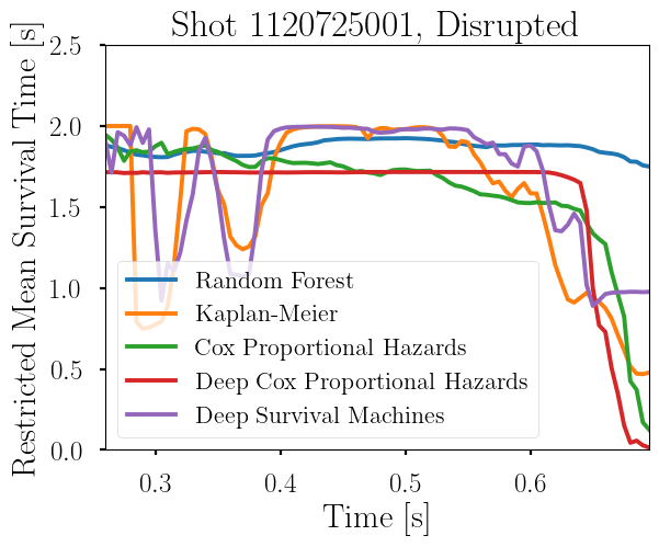
Once the survival functions are obtained, the expected time to disruption is calculated through the restricted mean survival time (RMST): \(RMST(\vec x) = \sum\limits_{n=0}^{2/\Delta t} S(\vec x, n\Delta t) n \Delta t\).
This is essentially a weighted average of the predicted probability that no disruption will occur over the course of many time intervals. The results of these three models predicting expected time to disruption on a shot from Alcator C-Mod is shown below.

It must be noted that the models were not explicitly trained to produce good output in a plot like this. The models as shown are trained to minimize misclassifications for each feature vector in the training set, and hyperparameter tuned for good shot-by-shot performance on a validation set. While a perfect model would do well in all cases, the metrics we are evaluating performance on are not yet aligned with calculating expected time to disruption. The next step of the project is designing workflows to train, tune, and test survival analysis models with metrics that are relevant to tokamak operation and with potential application to SPARC disruption avoidance.
The survival analysis team is led by graduate student Zander Keith (MIT NSE), with the close collaboration of Chirag Nagpal (Google) and Alex Tinguely (MIT). Zander’s supervisor is Dr. Cristina Rea.
References:
- [Rea2019] C Rea et al 2019 Nucl. Fusion 59 096016 doi:10.1088/1741-4326/ab28bf
- [Tinguely2019] R A Tinguely et al 2019 Plasma Phys. Control. Fusion 61 095009 doi:10.1088/1361-6587/ab32fc
- [Nagpal2021] C Nagpal et al 2021 “Deep Survival Machines: Fully Parametric Survival Regression and Representation Learning for Censored Data with Competing Risks”, doi:10.48550/arXiv.2003.01176
- [Nagpal2022] C Nagpal et al 2022 “auton-survival: an Open-Source Package for Regression, Counterfactual Estimation, Evaluation and Phenotyping with Censored Time-to-Event Data”, Proceedings of Machine Learning Research 182